Uber Badge Puzzles

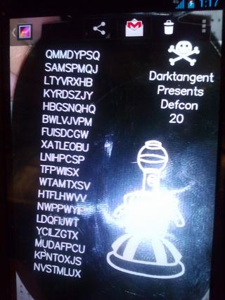
It was a normal weekend for me -- sitting at my computer, looking out from my second story apartment window as cars came and went; glancing inquisitively back and forth between my monitor and my newly acquired prize. My team (MLF) had won the badge challenge at Defcon 20 and I had received an Uber badge as the prize. This year, the badge featured a puzzle on its reverse, to be solved after the con by curious hackers. I had been working on the puzzle on and off since the con but had made no progress yet. It was November, and I was on the verge of a breakthrough.

One Time Pad

The One Time Pad (OTP) is a simple theoretical cipher system in which a plaintext is encrypted by a random one-time-use key of equal length to the plaintext. The ciphertext is calculated using an invertible function (generally modular addition or bitwise XOR) that is applied byte by byte (or character by character) in order to combine each plaintext byte with its corresponding key byte (c[i] = (p[i] + k[i]) mod 26). The system achieves perfect security if the key is truly random and is never reused; that is, decryption is absolutely impossible given only the cipher text. This is easily demonstrable: For any given OTP ciphertext and arbitrarily chosen plaintext of equal length, it is trivial to generate a key of length equal to the ciphertext that, when used to decrypt the ciphertext, would result in the chosen plaintext. It is impossible to validate potential decryptions without knowledge of the original plaintext.

In practice, OTP is impractical: storage and protection of the key is unruly for any real applications. Rather, many stream cipher systems such as RC4 attempt to emulate OTP by using Pseudo-Random Number Generators (PRNGs) to approximate a random key.

Running Key Cipher

Another play on OTP is the Running Key Cipher (RKC). In RKC, a non-random stream is chosen as the key such as a sentence or passage from a book or song lyrics. Like OTP, the ciphertext has no similarities to the plaintext except in length; and without knowledge that the text was encoded with a non-random key, the perfect secrecy properties of the cipher remain in-tact: given a cipher text, any key can be generated to produce a chosen plaintext. Unlike OTP, it is easy to rule out invalid plaintexts since their corresponding keys will likely not be intelligible.

This is the weakness of RKC: Given a ciphertext that was generated as a combination of two natural language texts, knowledge of the statistical model of the used plaintext and key languages is sufficient for decryption.

It is worth mentioning here that in RKC, it is generally true that decryption of the ciphertext using the key will result in the plaintext, and decryption of the ciphertext using the plaintext will result in the key. Because both key and plaintext appear as readable text, it is impossible beyond intuition to know which the cipher creator intended as the plaintext and which they intended as the key – intuition would select the more familiar text as the key. (Technical aside: this is true if an abelian function is used for encryption such as addition or XOR where A + B == B + A. Matrix multiplication, for example, may not have this property).

Cribbing

A common attack on RKC is cribbing. Given the knowledge that both the plaintext and key are, for example, English; it should be possible to choose a word or phrase that one believes is likely to appear in the plaintext (or key) and iterate over the ciphertext looking for decryptions that appear to also be English. When a promising decryption is found, the crib and its decryption are accepted as candidates for the plaintext and key. Additionally, in the likely event that word boundaries do not line up in the plaintext and key, it may be possible to derive additional characters by completing partially decoded words or phrases (e.g. “migh” will likely be followed by “t” possibly “ty”; “once upon a” could be followed by “time”). By repeating this process, it may be possible to discover large portions of the plaintext and key. Combining results across many cribs, one will eventually derive the plaintext.

To my dismay, this approach resulted in only small disconnected words and bits that appeared to be – but weren’t quite – English. This process was slow and I didn’t have any way to automate it.

Language Models

I had just graduated with my Masters in Computer Science and moved to California to start working. Most of my possessions were still packed away in boxes that lined my living room and I hadn’t yet had a reason to unpack most of them, especially my college text books. I had taken a number of courses focusing on machine learning and artificial intelligence, and I was fairly certain that I’d worked on similar problems in those classes; so I began looking.

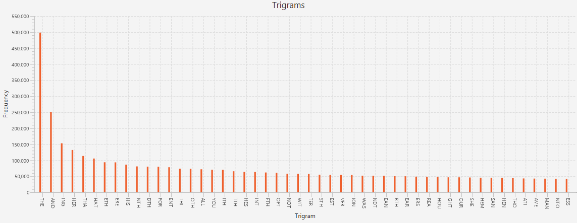
In Natural Language Processing applications (such as spell checkers and predictive text), language models are the core building blocks that store statistical information about the language they represent. Such models can be used to calculate probabilities of what was meant given what was typed or what will be typed next given what was typed previously. The N-gram model is one such model, used for calculating the likelihood of an N-gram (or sequence of N events, i.e. characters) based on how frequently that N-gram occurs in common use. It can be built relatively painlessly: given a set of English texts, one simply iterates over each text and records how frequently each sequence of N letters occurs.

I downloaded a set of English texts from Project Gutenburg and chose N = 6. Before too long I had a frequency tree that I could efficiently query for N-gram frequencies. To calculated the probability of a given N-gram, simply divide the number of times a given N-gram was observed by the total number of N-grams observed (#(N-gram) / #(.) ). From here, I could estimate the probabilities of strings longer than N using conditional probability chains, for example: P(c1c2c3c4c5c6c7c8) = P(c1)*P(c2|c1)*P(c3|c1c2)*P(c4|c1c2c3)*P(c5|c1c2c3c4)*P(c6|c1c2c3c4c5)*P(c7|c2c3c4c5c6)*P(c8|c3c4c5c6c7) where P(Y|X) = P(XY) / P(Y) = #(XY) / #(Y). Notice that since N = 6, my frequency tree only contains information for N-grams up to 6 characters long; so I can only calculate conditional probabilities for a character given its five previous characters (e.g. P(f | abcde) = #(abcdef)/#(abcde)). In effect, I am making a 5th order Markov Assumption: that the probability of a character in a string is dependent only on the 5 preceding characters.

With my model running, I was now able to efficiently sort crib decodings by “English-ness” and could run through dictionaries to identify the most probable words. Unfortunately, this method was still limited as the average English word length is just over 5 characters and the quantity of short decodings that were unintelligible almost-English was still too high.

Hidden Markov Chains and the Viterbi Algorithm

Twiddling my pencil, I attempted to recall some of the homework problems from my Machine Learning and Bayesian Probability courses. Consider that there exists a series of observations that are the results of an equal-length series of hidden events. It is possible to calculate the most probable series of hidden events that caused the observations if the underlying state-transition probabilities for those hidden events are known. Such a model is known generally as a Hidden Markov Model (HMM) and the class of problems that aim to uncover the most likely series of hidden events is called Most Probable Explanation (MPE). If I could represent the ciphertext and its underlying plaintext-key pair as a HMM, I would be able to use a dynamic programming algorithm known as the Viterbi Algorithm to solve it.

In RKC, the ciphertext characters are individually computed by adding corresponding plaintext and key characters together and are not otherwise related to each other. On the other hand, because the plaintext and key are both English, transitions from character to character are expected to follow English statistical models. Intuitively, it is more likely for the letter T to be followed by H than by G.



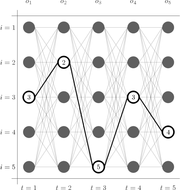
In the generalized Viterbi Algorithm, the goal is to compute the optimal path through a directed acyclic graph of U x V nodes (states) where U is the number of observations (length of the ciphertext) and V is the number of unique states (size of the alphabet = 26). Conceptually, the nodes are arranged in a series of U columns of V nodes each. Directed edges exist between every pair of nodes (states) from one column to the column immediately to its right with weights equal to the state transition probability, i.e. P(event | previous events). A brute force attempt at enumerating every path would result in O(M^N) paths – that’s over 100 trillion possible paths for just a 10 character cipher text. Viterbi is a dynamic programming algorithm, meaning it retains information as it computes to void duplicating calculations. Column by column, Viterbi computes the probability of being in each target hidden state by iterating over the previous column’s results and identifying the most likely previous state, taking into consideration (1) the probability of being in that previous state, (2) the probability of transitioning from that previous state to the target state, and (3) the probability of the target state given the corresponding observation.

To apply Viterbi to RKC, we need to identify how these calculations are to be applied. For (1), the probability of being in the previous state requires the identification of initial state probabilities. For RKC, we can use unigram probabilities. For (3) the probability of the target hidden state given the corresponding observation is 1 since the hidden states (key character and plaintext character) deterministically combine to result in the observation (plaintext character). Finally, for (2), since the transition probability is a combination of the two separate hidden states (the plaintext and the key). For each of these, we use the N-gram model to compute transition probabilities and multiple their results together.

At the completion of the Viterbi Algorithm, the path is traced backwards from the most probable final state in order to identify the most probable path. This path is the most probable explanation for the ciphertext and the solution.

Eureka

The feeling of accomplishment as I began seeing words and phrases appear out of nothing was euphoric. The decryption wasn’t perfect, but gave me enough that I could begin searching the web for potential key texts. Upon stumbling upon a Mystery Science Theater 3000 fan site, I had what I needed. The rest is history.

Prologue

Fast forward three years. Defcon 23 has concluded and the hackers have begun their journeys back home. MLF did not win the badge challenge, but I’m still feeling the itch. As I line up to board my flight back to the East coast, I notice that 1o57 is on my plane and I remember the cipher etched in this year’s Uber Badge coin. As the plane climbs to 10,000 ft, I crack open my laptop and transcribe the cipher text into my program’s input. Seconds later, I have a 90% solution – plenty enough to recover the original key from an online search. I write the solution on a scrap of paper and hand it to 1o57 as I deplane.

Errata

I’ve left out some fairly important implementation details that should be considered should you attempt to recreate my program.

1) Probabilities become very small when repeatedly multiplied. To avoid underflows, one should use log-probabilities. (Recall: log(P(x) * P(y)) = log(P(x)) + log(P(y))

2) In practice, there are occasions when a character sequence has never been seen. Rather than using a frequency of 0 (which tends to throw off other calculations; 0*X = 0), in these cases I hard code a small constant value epsilon.

3) My implementation of Viterbi uses N-grams as its unit of state (V = 26^N) but only retains the top 100,000 probable previous states for consideration in the next state calculation. This was a performance / accuracy trade off that can be dialed up or down. There are probably other (better) ways to extend Viterbi to N-degree Markov, but this was my approach that seems to work (at least somewhat).

4) I originally wrote my code in Python and rewrote it in Java. Java is significantly faster (but only by a factor of ~2-4. I intend to reimplement in C... will report back :)